next example
Spectral Library
Ensemble Support Vector Regression
SVR uses a library of reference surfaces and unmixes image pixel spectra into fractions of those references.
Library spectra are selected from heterogeneous areas in the Landsat images.
We select 10 reference spectra for each of the 4 classes and 5 years.
Using a total of 200 reference spectra, we compute 1200 training sets of artificial mixtures in steps of 20%.
Those help to determine gradual surface information using a regression algorithm.
This is the input to our SVR model.
Hover over a surface mixture visualize spectral mixing in the chart to the left.
0
100
0
100
0
20
80
0
80
0
0
80
20
80
20
40
60
0
60
0
20
60
20
60
20
0
60
40
60
40
60
40
0
40
0
40
40
20
40
20
20
40
40
40
40
0
40
60
40
60
80
20
0
20
0
60
20
20
20
20
40
20
40
20
40
20
20
60
20
60
0
20
80
20
80
100
0
0
0
0
80
0
20
0
20
60
0
40
0
40
40
0
60
0
60
20
0
80
0
80
0
0
100
0
100
SVR is a Support Vector Machine method designed to solve regression problems. It uses non-linear kernel transformation in order to map input data into a higher dimensional feature space and, then, applies a linear regression model solving
higher dimensional problems
 .
.
.
In an examplary case with two simple classes and clear feature distinction, SVR can easily separate the data.
The method finds a simple function to separate one class from the other.
separate data in 2D
In our case of various and complex classes, visualization is harder, because class separation
is not linear. SVR translates all data in a higher dimensional (here: 3D) space using a kernel function.
separate data in 3D
Class separation is now easier using a linear plane. SVR finds the plane and re-projects the data back in a 2D space, now being able to separate
the more complex dataset.
mapping urban expansion
in a west-african city
in a west-african city
Ouagadougou
Burkina Faso
Using Ensemble Support Vector Regression on Landsat time series for urban pattern quantification.


Population
Burkina Faso
Ouagadougou
Urban Primacy
Burkina Faso is one of the fastest growing countries on earth. Reaching about 18 million inhabitants in 2016,
the Sub-Saharan West-African state quadroupled its population since 1950. Projections say that this trend is about
to continue until the end of the century. Immigration from surrounding areas and natural growth (above 30‰, - among the
TOP 15 worldwide, can be considered Reasons for this growth, along with many other.
Ouagadougou features one of the largest rates of population growth worldwide. From 1980 to today, the number of inhabitants increased by more than 1000 %.
Hover the bars and compare this number with other agglomerations in Africa and Europe. Although Sub-Saharan Africa is a region with low degrees of urbanization, rural-urban migration may be one of the many reasons.
Urbanization tendencies within the last decades increase the importance of Ouagadougou as a primate city. About 15% of the country's population
lived here in 2015. In that regard, Burkina Faso's second largest city, Bobo-Dioulasso, is stagnating.
Burkina's urbanization rate catches up with averages in Western and Sub-Saharan Africa.
Urban development patterns
Very high resolution satellite imagery reveals that the character of growth within the city is diverse.
Formally planned settlements stand out through highly systematic infrastructural networks under municipal supervision, defined architectural specifications and documented lot ownership.
Go through the examples to discover more attributes of planned settlements!
Photo: J. Hauer
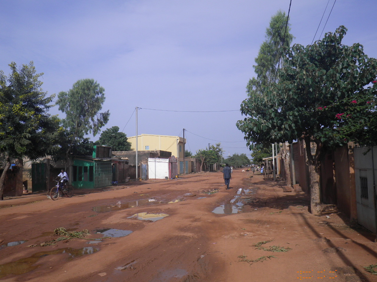
Urban development patterns
Unplanned settlements, however, develop beyond official planning strategies. They feature more diverse processes of property conveyance, building layouts and an unsatisfactory consideration of public services, such as water, electricity or roads.
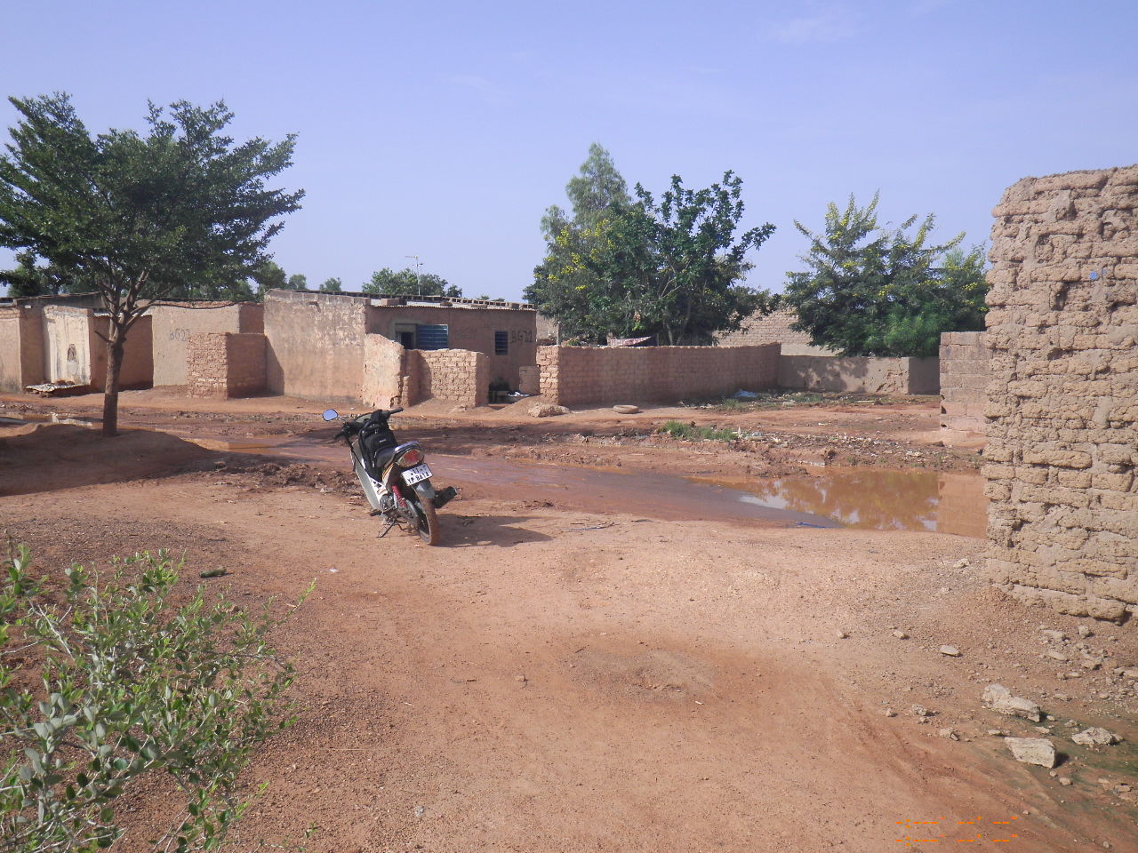
Go through the examples to discover more attributes of unplanned settlements!
Photo: J. Hauer
Landsat satellite images
This study uses data from the Landsat satellite mission.
Landsat is a multi-spectral NASA-operated earth observation satellite, orbiting our planet in various technological iterations since 1972 and offers
the largest free-to-use database of satellite imagery.
Landsat scans every spot on earth every 16 days, one image is approximately 180x180 km in size.
Low secondary data availability makes satellite images increasingly useful for land cover monitoring.
The Landsat footprint map reveals inequalities in image availability.
As there are limitations in downloading data from satellites, those are mainly due to regional priorisation.
We used the following images from dry (red) and rainy (blue) season:
In order to work with data from similar phenological states and to achieve comparability, we select images based on
an averaged image vegetation index NDVI.
Classification
Landsat does not feature a very high spatial resolution sensor. Its pixel size of 30x30 meters is a challenge in urban areas and leads
to a mixed pixel problem, meaning that one pixel contains multiple urban structures.
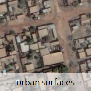
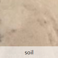
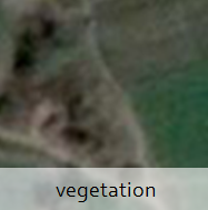
Instead of visual interpretation, spectral information can be used for land cover mapping. Besides three red/green/blue channels, Landsat features three bands in the near infrared spectrum.
Hover over the snippets to see how surface classes look like in Landsat and what their typical spectrum is.
Landsat satellite images
Despite its resolution, Landsat is still able to give a visual impression of Ouagadougou's expansion since the 1980s.
Use the slider in order to travel through time! Use a false color interpretation to display data using Landsat's infrared bands.
Show a false color representation using both the visible and infrared spectrum
1986
In 1986, Ouagadougou is significantly smaller than today. There was no built-up area north of the great reservoir
and today's inner-city ariport was located in the urban periphery.
In false colors, red is an indicator for vegetation because of its infrared reflectance. Urban surfaces appear in blueish colors,
wheras green and white colors represents open surfaces.
2002
In 2002, the urban core of Ouagadougou is surrounded by a belt of more or less long-established and planned
neighborhoods. In the urban fringe, urban expansion can be anticipated on areas covered with bare soil.
The overall high level of red color shows that in comparison to 1986, phenology was at a slightly more advanced state when the image was taken.
2007
In 2007, urban expansion focuses on the north-west, south-west and south-east of Ouagadougou. We detect ongoing
development in Ouaga 2000, a recent city expansion from scratch, including the new Palais de Kosyam, the president's seat.
2009
In 2009, parts of the business district close to the international airport have been demolished for re-development.
We observe rapid growth in the western part of Tampouy, and further expansion highlights the presence
of an urban green belt.
2011
Less rapid and apparent grwoth occurs between 2009 and 2011.
Due to atmospheric or phenological influences, surrounding landscape appears slightly different.
2013
Redevelopment becomes now obvious in the central airport district. We observe densification and further expansion in the outskirt areas.
Open soil areas indicate future growth, whereas we can observe the annexation of former independent
settlements into the greater Ouagadougou area.
Climate
Ouagadougou is located in a semi-arid savannah region. Regional climate is characterized as tropical summer-humid under the influences of
an ITCZ driven rainy season from May to September with slightly lower temperatures and high precipitation
a trade wind driven dry season from October to April with high temperatures and little precipitation
Visualize differences in vegetation, precipitation and temperature during dry and rainy season!
Vegetation
Precipitation
Temperature
Display the difference between one dry season and one rainy season Landsat image!
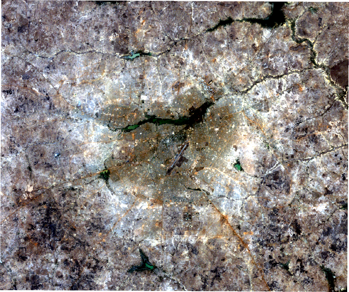
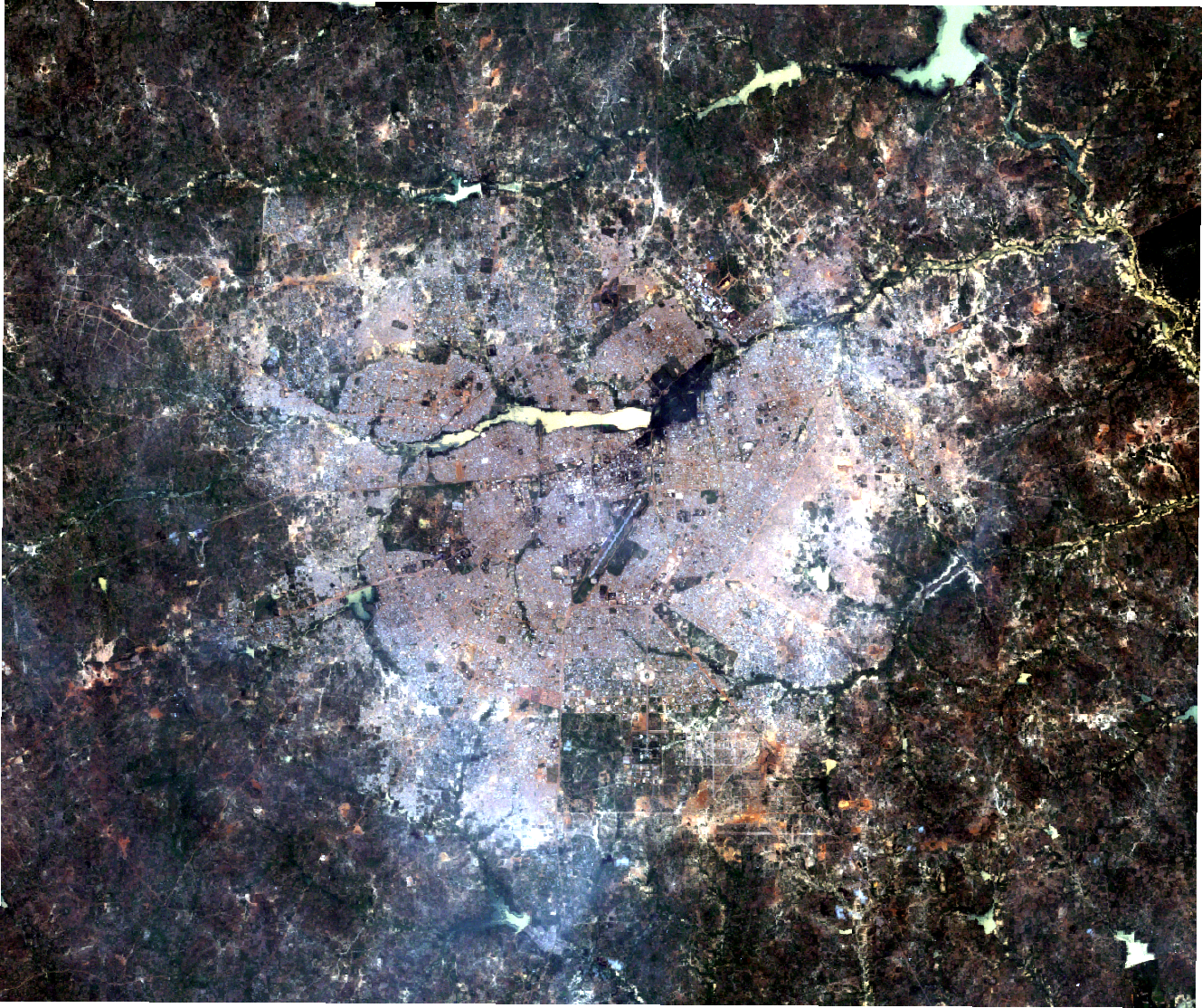
Dry/rainy season Landsat imagery
Climatic differences affect the visual impression of the earth's surface, but also spectral attributes.
January (dry season)
August (rainy season)
Methodology
We use Support Vector Regression (SVR) to map urban surfaces.
SVR can extract sub-pixel information by calculating land cover fractions for each pixel and allows
statements about gradual urban develpoment.
SVR accounts for the spectral variability within and among surface classes.
SVR is flexible regarding input data. We introduce a new class, seasonal vegetation, to cover areas that are soil or
vegetation in different seasons.
Select up to three surfaces and see how a seasonal dimension adds spectral information to the data that would be hidden in a single image!
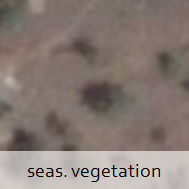
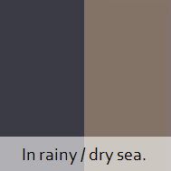
Seasonal vegetation's spectrum is similar to soil during dry and similar to vegetation during rainy season, whereas
all other surfaces are consistent during the year.
Results
The first major result of our classification is a map of historic urban expansion. The color indicates the year in which we could identify relevant urban area in a pixel. The shading represents the fraction of urban surface in 2013, the last year of this study.
Hover over the map to see urban fractions at each pixel for the all years.
Urban surfaces first exceeded 20% coverage within a pixel in
Whereas in the urban core, urban settlements have been established for a longer period, we observe temporal
patterns of development in the outskirt areas.
Results
The second major result of the study is the delineation of different types of neighborhood development.
We found out that bi-seasonal image information is beneficial here. The ratio of seasonal vegetation to open soil fractions
is appropriate to indicate whether a neighborhood is characterized by rather unplanned (green) or planned (red) development.
Hover over the squares to get information about each example.
This is an example of a planned neighborhood.
This is an example sentence.
Result quality
We use systematic validation to evaluate result quality.
Within the city, we use seven validation areas similar to the one on the right.
For each point, we manually extract land cover reference data from high res. images.
We use a total of 15.435 reference points over five time steps and all areas.
Fractions from modelled maps are compared to the reference land cover fractions.
Hover over the reference points within the validation pixels to see how that works for a specific example!

Averaged Mean Absolute Error (MAE) values show that the applied model produces generally good quality results.
| Urban surfaces | Vegetation | Soil | Seasonal vegetation | |
| MAE | 0.10 | 0.14 | 0.10 | 0.13 |
Further Information
This website represents research highlights from a research article and has been developed by the first author for
demonstration purposes. The website translates information in a very condensed and potentially unscientific form for accessibility.
Check the article that this website is based on to find out more!
F. Schug
 , A. Okujeni ,
J. Hauer ,
P. Hostert ,
J. Ø. Nielsen ,
S. van der Linden .
2018. Mapping patterns of urban development in Ouagadougou, Burkina Faso, using machine learning regression modeling with bi-seasonal Landsat time series, Remote Sensing of Environment, Vol. 210, pp. 217 - 228,
https://doi.org/10.1016/j.rse.2018.03.022
, A. Okujeni ,
J. Hauer ,
P. Hostert ,
J. Ø. Nielsen ,
S. van der Linden .
2018. Mapping patterns of urban development in Ouagadougou, Burkina Faso, using machine learning regression modeling with bi-seasonal Landsat time series, Remote Sensing of Environment, Vol. 210, pp. 217 - 228,
https://doi.org/10.1016/j.rse.2018.03.022
Further reading
Fournet et al. (2008)
, Beauchemin (2011)
and Hauer et al. (2018)
might serve as a starting point for understanding specific aspects of Ouagadougou as a study area.
Small (2005)
discusses the usability of Landsat data for urban areas in general, whereas Griffiths et al. (2013)
and Taubenböck et al. (2012)
apply remote Sensing
techniques to urban monitoring. Knauer et al. (2017)
is an example for previous remote sensing work in Burkina Faso.
Okujeni et al. (2016)
is the methodological basis for this study and Dudley et al. (2015)
contributes to understanding the importance of seasonality in spectral libraries.